Day 1 - Why Do We Need an ML Compiler?

You trained a model and it runs fine in PyTorch. But once it goes to production, inference is slow and expensive. On the very same GPU, someone else is running two or three times faster. Where does the difference come from?

Often the answer is simply this: they use a compiler, and you are still running plain eager mode.

This series will take torch.compile, TVM, TensorRT-LLM, and vLLM apart one by one. But before touching any tool, there is a more basic question to answer: what is a compiler actually solving? This post covers no framework at all. It only makes that question clear, because it is the common ground for understanding everything that follows.

It Starts With Frameworks and Hardware Wanting Different Things

On the framework side, PyTorch gives you flexibility. You write Python, it executes line by line, you print whenever you want, you drop in an if whenever you want. This "write a line, compute a line" model is called eager mode. It makes development and debugging comfortable.

On the hardware side, a GPU wants something completely different: one big chunk of work that fills thousands of cores and does not shuttle data back and forth.

These two expectations conflict. The convenience of eager mode is paid for in performance. The cost is just usually well hidden.

The Three Hidden Costs of Eager Mode

Look at a perfectly ordinary piece of code:

# eager mode: every line is its own GPU kernel
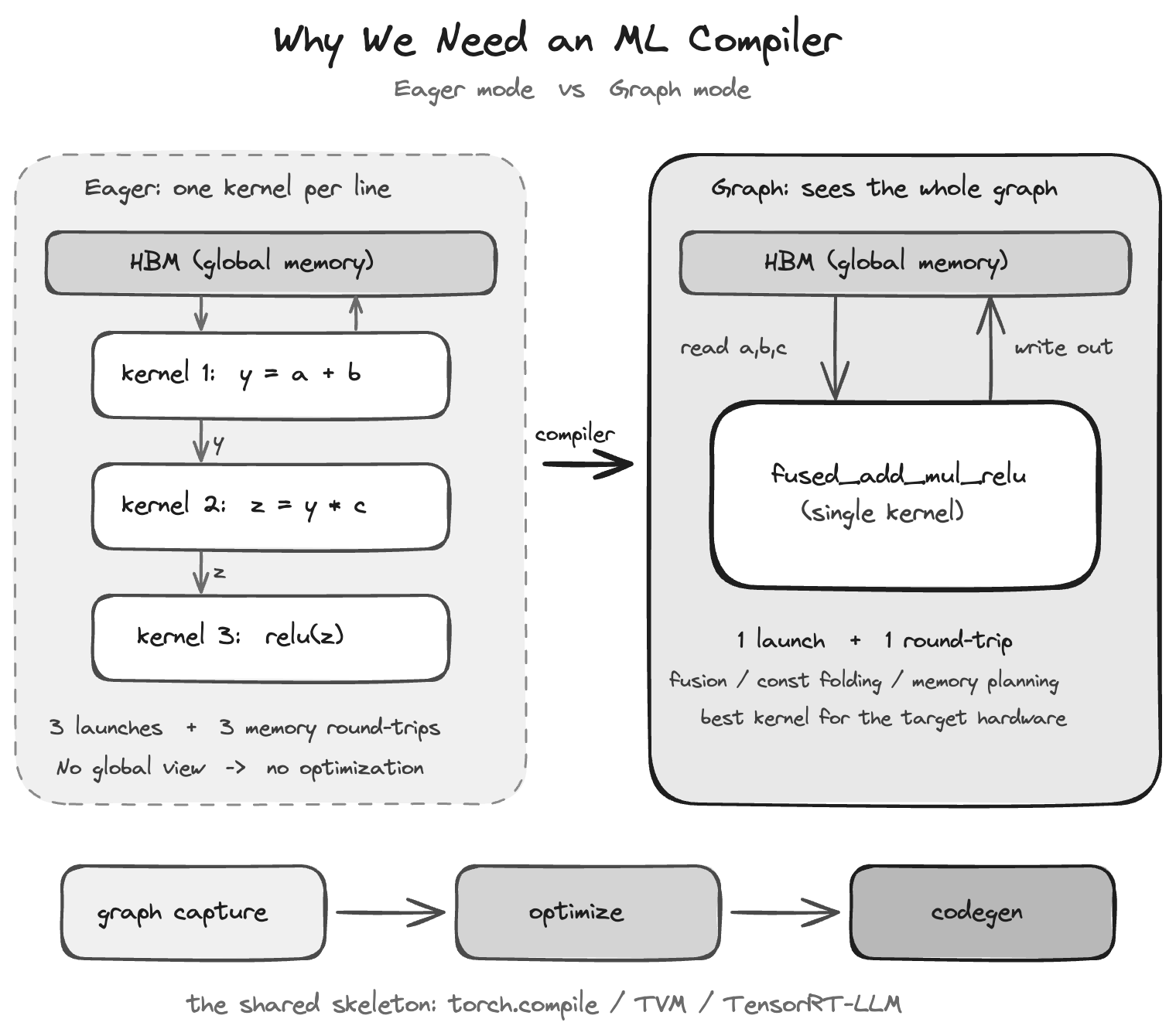
y   = a + b       # kernel 1: read a, b -> compute -> write y
z   = y * c       # kernel 2: read y, c -> compute -> write z
out = relu(z)     # kernel 3: read z    -> compute -> write out

Three lines, three hidden costs:

1. Kernel launch overhead Every op goes through Python dispatch first, then launches a GPU kernel. Launching itself carries a fixed cost. The more ops you have, and the smaller each one is, the larger a share this overhead takes.

2. Memory round-trips, this is the important one. Every kernel reads its data in from the GPU's global memory (HBM), computes, and writes the result back out. Intermediates like y and z above are needed by the very next step, yet they get dutifully written back to HBM and read out again. For many computations the real bottleneck is not how fast you compute but how fast you move data. We call this being memory-bound.

3. No view of the whole Eager mode executes one op at a time and never knows what comes next. Since it cannot see ahead, it cannot perform any optimization across ops.

Graph Mode: Understand the Whole Picture First

What if we do not rush to execute, and instead "record" the entire computation into a graph?

Once you hold the whole graph, you can see its structure, and that opens up plenty that eager cannot do:

• Operator fusion: merge a+b, *c, and relu into one kernel. Read the data once, compute all the way through, write once. Three memory round-trips become one.
• Dead code elimination and constant folding: on the graph you can see which computations are redundant and which results can be computed ahead of time, at compile time.
• Memory planning: knowing the full lifetime of every buffer lets you plan how to reuse them.
• Picking the best kernel for the hardware: the fastest implementation of the same matmul differs across GPUs, and you need the whole picture to choose well.

After fusion, it conceptually looks like this:

# after the compiler fuses: one kernel does it all
out = fused_add_mul_relu(a, b, c)   # read a, b, c -> compute -> write out

The difference in one sentence: eager sees a single leaf of a tree, graph sees the whole tree. Almost all room for optimization comes from being able to see the whole picture.

This Is What an ML Compiler Does

Putting it together, an ML compiler is essentially three steps:

1. Graph capture: turn the model into a graph.
2. Optimize: apply fusion, layout transforms, memory planning, and more on the graph.
3. Codegen: emit efficient executable code for the target hardware.

It stands between the high-level flexible framework and what the hardware actually wants, and closes the gap between them.

This path, graph, optimize, codegen, is the shared skeleton of every tool that follows. torch.compile, TVM, and TensorRT-LLM all walk it. They differ only in which segment they make especially strong, and which hardware and workloads they serve. Remember this skeleton and every framework you look at becomes the same set of questions: at which layer does it capture? which optimizations does it run? who does it generate code for?

Why It Matters Now, in the LLM Era

Compilers are not new, but in recent years they went from nice-to-have to near-mandatory, for two reasons:

• Scale is money: LLM inference is expensive. At the scale of millions or tens of millions of requests, every 10% saved shows up directly on the bill. At that volume, it is worth spending engineering effort to squeeze out performance.
• LLM inference is heavily memory-bound: especially during decode, where one token comes out at a time. The actual arithmetic is modest, yet enormous weights and the KV cache have to be moved constantly. That lands squarely on what compilers are best at, and it is the main battleground for fusion, quantization, and KV cache management.

This is why the inference framework ecosystem suddenly exploded: torch.compile, TVM, TensorRT-LLM, and vLLM are all racing to close that gap, just entering at different layers. Telling apart which layer each one stands on is the map this series wants to build for you.

Next

This post answered the "why". The next one (Day 2) draws the conceptual map of "how": what an IR is, why a compiler needs several layers, how a model gets lowered step by step, and what codegen actually generates. That map will be the shared language we use to take apart each tool later.