Day 2 - IR, Multi-Level Lowering, and Codegen

On Day 1 we arrived at a skeleton: compiler = capture, optimize, codegen.

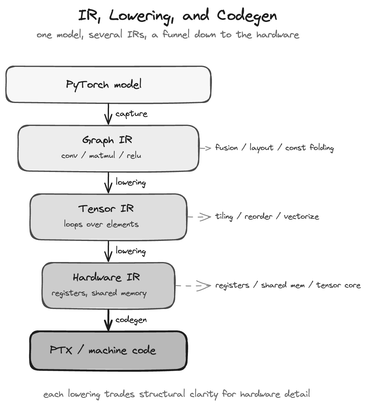
But something was left unsaid. That graph in the middle is not one thing. Along the way, a real compiler turns your model into several different forms, lowering it one level at a time. Understanding these levels is the single most useful mental model for reading any compiler, and this post draws that map.

What Is an IR?

IR = Intermediate Representation, the data structure a compiler uses internally to represent your program. It is not Python and it is not machine code. It sits between the two, designed specifically to be easy to analyze and rewrite.

An analogy: to translate a book from Chinese into Japanese, a good translator does not swap words one by one. They first turn the text into a layer of "meaning" in their head, then write fresh Japanese from that meaning. The IR is the compiler's layer of "meaning". Your PyTorch program is friendly to humans, machine code is friendly to the GPU, and the IR is the workspace in between where the compiler does its work.

The graph from Day 1 is one kind of IR. But here is the key: there is more than one IR.

Why Multiple Levels of IR?

This is the most important idea in this post. Once you have a graph, why not just do every optimization on it and be done?

Because abstraction levels come with a trade-off:

• High-level IR (nodes are whole ops like conv, matmul, relu): you can see the model's structure at a glance, which suits fusion, choosing data layouts, and algebraic simplification. But it hides how each op is actually computed.
• Low-level IR (loops, indices, individual memory accesses): you can see the real loop structure, so you can tile, vectorize, and map work onto GPU threads. But you can no longer tell that this pile of loops is a matmul.

No single representation does both kinds of optimization well. So the compiler's strategy is: stop at the high level first and do the optimizations that belong there; then lower into a finer form and do the optimizations that belong at that level; and so on, down through the levels.

Take a matmul followed by a relu and watch it transform level by level:

Level one: graph IR (nodes are whole ops)

%1 = matmul(%x, %w)
%2 = relu(%1)

What this level can do: fuse relu into the tail of matmul, decide which layout %x uses, fold away constants that can be computed at compile time.

Level two: tensor IR (each op expands into loops over tensor elements)

for i in range(M):
    for j in range(N):
        acc = 0
        for k in range(K):
            acc += X[i, k] * W[k, j]
        Y[i, j] = max(acc, 0)   # relu is fused in

What this level can do: tile the loops to fit in cache or shared memory, reorder them, vectorize, map i and j onto different threads. Notice that by now you can no longer see "this is a matmul". All that is left is a set of loops to sculpt.

Level three: hardware IR: the tiled and scheduled loops above get mapped onto real hardware resources, registers, shared memory, even tensor cores.

Each level down, you trade structural clarity for hardware detail. That is why the levels exist.

What Lowering Is

Lowering is the process of converting a program from a higher-level IR into a lower-level one. Each lowering reveals more implementation detail while discarding some abstraction.

The optimizations within each level are usually implemented as individual passes: a pass reads in an IR, rewrites it, and emits the rewritten IR. A compiler's optimization power is largely a matter of which passes it has and how they are chained.

So the whole pipeline behaves like a funnel: the model enters at the wide, abstract top, gets rewritten, lowered, and narrowed all the way down, and something executable flows out the bottom.

What Codegen Actually Generates

Codegen is the last step: turning the lowest-level IR into something the target hardware can really run.

What that something is depends on your target:

• GPU: CUDA C or PTX, or generated through Triton and then turned into machine code by LLVM.
• CPU: usually lowered to LLVM IR, with LLVM generating the machine code.

The point is that codegen knows the hardware. The same low-level IR can produce one kind of code for a GPU, another for a CPU, and yet another for a phone or an accelerator. This is why one model can be compiled to run on so many different platforms.

And its output is clean native code, no Python, no per-op dispatch overhead, just something you can feed the hardware to run at full speed. That lines up exactly with the costs from Day 1: most of them get eliminated right here.

Drawing the Map

Put together, the whole path looks like this:

your model (PyTorch)
      │  capture
      ▼
  graph IR       ──►  fusion, layout, constant folding
      │  lowering
      ▼
  tensor IR      ──►  tiling, loop reorder, vectorize, map threads
      │  lowering
      ▼
  hardware IR    ──►  register / shared memory allocation
      │  codegen
      ▼
  executable native code (PTX / machine code)

This is the skeleton every tool that follows shares. A small spoiler, so you can place them when you meet them:

• torch.compile: Dynamo captures into the graph level, and Inductor carries the tensor level all the way through codegen (via Triton).
• TVM: Relax is its graph IR and TIR is its tensor IR, and it ships codegen for many backends.
• TensorRT-LLM: leans toward heavy optimization at the graph level, paired with highly tuned kernels.

For now it is enough to remember that every tool lives on some subset of these levels. The details belong to their own posts.

Next

This post covered which levels optimization happens at. The next one (Day 3) looks at what actually happens inside them: operator fusion, constant folding, layout transformation, and memory planning, the four core optimization techniques, what each one saves and why it works. With the map in hand and these moves recognized, we will be ready to open up the first real tool.