Day 3 - The Four Core Optimizations | Guan-Ming (Wesley) Chiu

The four core optimizations against the two enemies of performance

The first two posts established two things: Day 1 explained why compilers exist, and Day 2 mapped out which levels optimizations happen at. This post fills in the last piece: what those levels actually do.

Compilers have many tricks, but most of the speedup comes from a handful that show up over and over. This post picks the four core ones. Once you can recognize them, you will find that the docs and release notes of almost any tool are really saying "we made these same few things more automatic and more thorough."

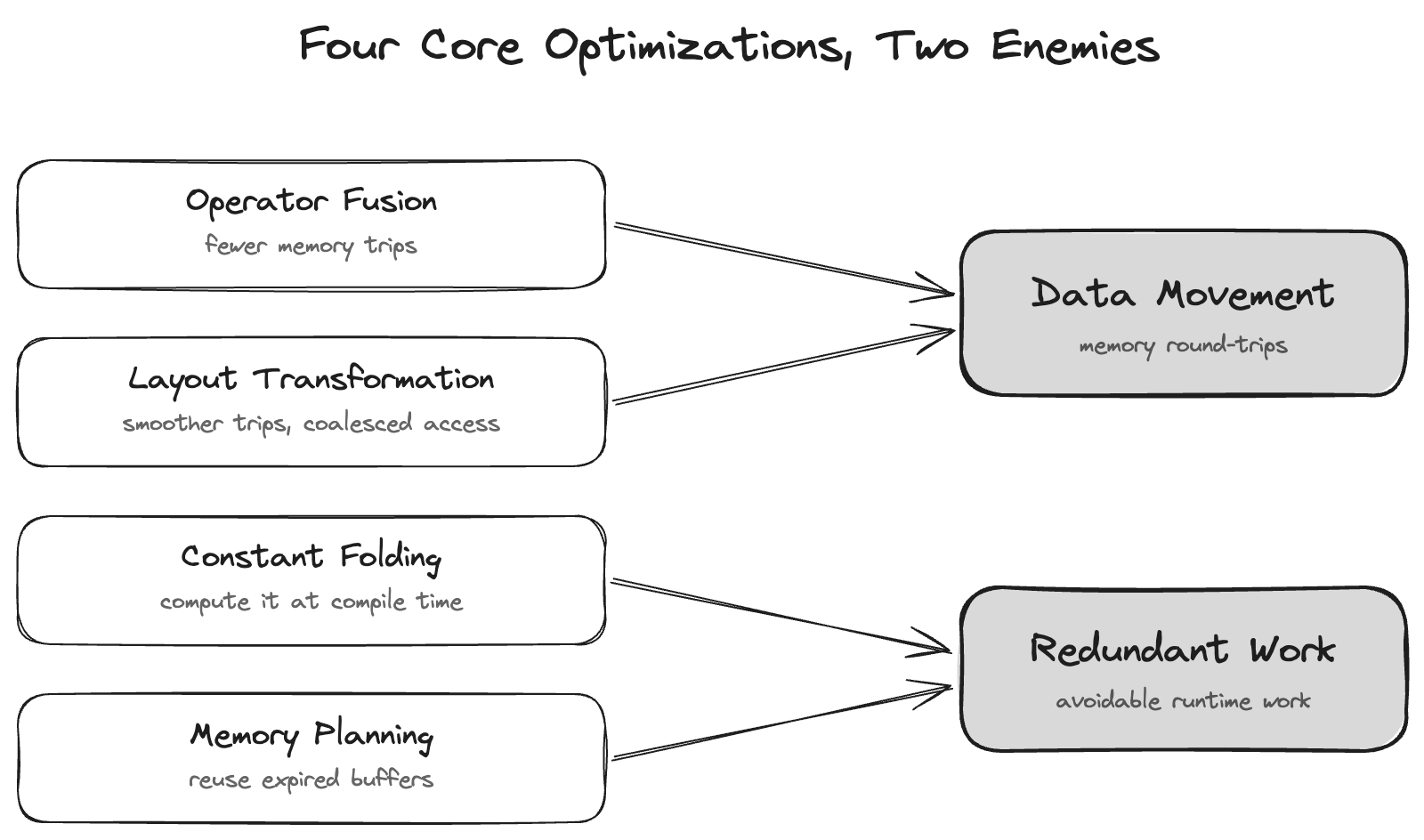
First, some orientation. Recall from Day 1 that the two great enemies of performance are data movement (memory round-trips) and redundant work. The four moves below essentially take turns fighting these two enemies.

1. Operator Fusion

One sentence: merge several consecutive small ops into a single kernel.

The a+b → *c → relu example from Day 1 is exactly this: three kernels and three memory round-trips originally, and after fusing into one, the data is read once, computed all the way through, and written once.

Two kinds of fusion are especially common in practice:

Chained element-wise fusion: a run of element-wise operations (add, multiply, activation, ...) gets merged into one kernel.
Epilogue fusion: the bias and activation that follow a matmul or conv get folded into the tail end of that heavy kernel, instead of launching separate kernels.

What it saves: memory round-trips plus kernel launch overhead. Especially sweet for memory-bound workloads (LLM decode is one). Which level it lives at: the graph level decides who fuses with whom; the tensor level generates the fused loop nest.

2. Layout Transformation

One sentence: decide how each tensor is arranged in memory.

The same tensor can be row-major, NCHW or NHWC, or some special tiled layout. Why does this matter? Because GPUs read contiguous memory fastest (coalesced access), and tensor cores prefer specific layouts. Get the arrangement right and the same amount of data moves noticeably faster; get it wrong and no amount of compute saves you from being stuck moving data.

An example: in a chain of convs, if every conv uses the hardware's preferred layout, there is no need to keep converting back and forth in between. The compiler weighs, globally, the cost of one layout conversion against the benefit every later step gains from it, then decides whether to insert a conversion and where it pays off most. This is exactly the kind of judgment that only "seeing the whole picture" makes possible.

What it saves: memory bandwidth, coalesced access, and sometimes it unlocks tensor cores. Which level it lives at: the graph level picks the layout; lower levels implement it.

3. Constant Folding

One sentence: anything that does not depend on the input and can be computed at compile time gets computed ahead of time.

The simplest example:

y = x * (0.5 * 2.0)     # the compiler precomputes 0.5 * 2.0 = 1.0
# after folding → y = x  # this multiply never happens at runtime

ML has a classic instance: folding BatchNorm into the preceding Conv at inference time. At inference, all of BN's parameters are fixed values, so its scale and shift can be merged directly into the previous conv's weights and bias. The result: the BN op disappears entirely, saving a whole operator in one stroke.

What it saves: runtime computation, sometimes an entire op. Which level it lives at: the graph level.

4. Memory Planning

One sentence: let tensors that are no longer needed hand their memory to later tensors for reuse.

Because the compiler sees the whole graph, it knows every intermediate tensor's lifetime: when it is produced and when it will never be used again. Knowing that, there is no need to allocate a fresh block for every intermediate result; once a tensor "expires", its space can go straight to a later tensor.

An analogy: parking spaces. When a car leaves, the next one pulls in. You do not build a new parking space for every arriving car.

What it saves: peak memory usage (the space saved can go toward a bigger batch or a bigger model), and fewer allocation calls. Which level it lives at: it needs whole-graph information → graph-level analysis.

Conclusion: Four Moves, Two Enemies

Put the four moves back against Day 1's two enemies and it becomes clear:

Cut data movement: Fusion (fewer trips), Layout (smoother trips).
Cut redundant work: Constant Folding (compute early what can be computed early), Memory Planning (reuse the space that can be reused).

With this, the conceptual trilogy, why, at which level, and doing what, is complete. These three posts are the foundation of the whole series: for every new tool you meet from here on, you can ask it three questions with this framework: at which level does it capture? which of these moves does it apply? and for whom does it generate code?

Key takeaways

The grouping is by what a move saves, not by what it touches. Memory Planning spends all day managing memory, yet what it eliminates is redundant work, allocation and peak occupancy, while the data still moves exactly as before. Layout is the one in the data-movement camp, because it makes the same volume of data move faster. To classify a move, ask "what cost does it cut", not "what resource does it handle".

Fusion is especially sweet for memory-bound work because it cuts at the bottleneck. In a memory-bound op, nearly all the time goes to waiting on data moving in and out of memory while the compute units idle; removing the intermediate round-trips shortens that whole span directly. In a compute-bound op, time is dominated by the arithmetic and the data movement already hides behind it, so removing trips barely moves the total. Same move, but it only pays when it lands on the bottleneck.

Next Up

Now that you know all four moves, which one should you reach for when facing a specific op? Day 4 hands you a ruler first: arithmetic intensity and the Roofline model. Measure whether an op is memory-bound or compute-bound, and you will know whether to cut data movement or cut computation. This ruler will come up again and again as later posts dig into each move.