This is the first post that digs into compiler optimizations in depth. Before drilling into any single technique, there is a prior question to answer: facing a given op, which kind of optimization should I even do?
Because more optimization is not better. Some ops barely speed up even with fusion and quantization all applied; others do not budge no matter how much data movement you shave off, because the real bottleneck is compute. Aim wrong and the effort is wasted. This post hands you a ruler for telling, at a glance, where to aim. It will be the shared yardstick for every deep-dive that follows.
Two Bottlenecks: Memory-Bound vs Compute-Bound
Day 1 named the two enemies of performance: data movement and redundant work. Flip that around, and a slow op is usually slow for one of two reasons:
- Memory-bound: the time goes to hauling data in and out of HBM, while the compute units mostly wait.
- Compute-bound: data arrives fast enough; the bottleneck is the arithmetic itself.
Here is the key: the same instruction, "go optimize this op", means completely different things for these two. A memory-bound op needs less data movement (fusion, quantization, layout); a compute-bound op needs a better kernel (tiling, tensor cores). The wrong medicine does nothing.
So how do you tell which kind an op is?
Arithmetic Intensity: One Ratio Decides Its Fate
Arithmetic intensity = the amount of computation an op does ÷ the amount of data it moves, measured in FLOP/byte.
It measures "how much computation you get per byte moved". A low ratio means lots of moving, little computing → memory-bound. A high ratio means each piece of data gets reused many times → compute-bound.
Run the numbers on two extreme ops (fp32, 4 bytes per element):
Element-wise add y = a + b (length N)
- Computation: about N additions
- Data moved: read a, read b, write y = 3N elements = 12N bytes
- Arithmetic intensity ≈ N / 12N ≈ 0.08 FLOP/byte → extremely low, unquestionably memory-bound
For an op like this, optimizing the "compute" is useless, because it spends almost no time computing. The only lever is fewer memory trips, which is exactly fusion's home turf.
Matrix multiply M×K · K×N (take a large square matrix of size n)
- Computation: about 2n³
- Data moved: about 3n² elements = 12n² bytes
- Arithmetic intensity ≈ 2n³ / 12n² = n / 6 → grows with n; large matrices are compute-bound
For a big matmul, saving data movement helps little, because it was never waiting on data. The real lever is doing the arithmetic more efficiently: tiling to squeeze the cache, using tensor cores. That is the home turf of Day 6 on loop scheduling.
The same word "optimize" tells one op to cut movement and the other to push compute. The difference hides in this one ratio.
Roofline: Drawing the Whole Picture
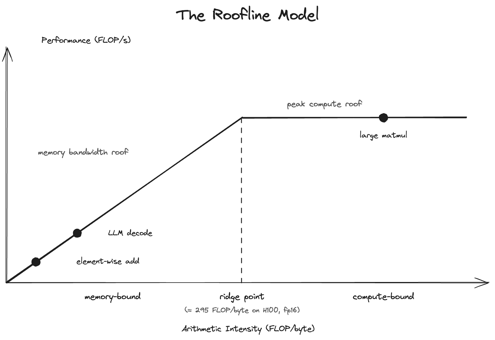
Put arithmetic intensity on the x-axis and achievable performance on the y-axis, and you get the famous roofline model at the top of this post.
First, the two axes. The x-axis is the arithmetic intensity from the previous section. The y-axis is the speed the op actually achieves (FLOP/s, floating-point operations per second): think of it as the speed on the dashboard once you floor the pedal. That speed has a ceiling, and the ceiling comes from two sources, whichever is lower:
- Peak compute (the flat roof on the right): the compute units can only do so many operations per second. A hardware spec, independent of your op.
- Bandwidth × arithmetic intensity (the slope on the left): if your op gets only x operations out of each byte it moves, and memory can feed only so many bytes per second, then the most you can compute per second is bandwidth × x. When data cannot arrive fast enough, the fastest compute units just sit and wait. Higher intensity raises this ceiling, which draws a line climbing up and to the right.
Take the min of the two ceilings and you get exactly that "slope meets flat roof" roofline. Where your op sits on the x-axis, and which section of roof it hits when it looks up, decides its fate:
- Left of the ridge point → it hits the slope → memory-bound → only movement optimizations help.
- Right of the ridge point → it hits the flat roof → compute-bound → only compute optimizations help.
Look back at the chart on top: element-wise add and LLM decode both hit the slope, throttled by bandwidth, nowhere near the compute ceiling on the right; only the large matmul reaches the flat roof and truly saturates the hardware.
The ridge point itself = peak compute ÷ memory bandwidth, a property of the hardware. This explains something important: the same op can flip from memory-bound to compute-bound when you switch GPUs, because every card has a different compute-to-bandwidth ratio, which moves the ridge point. This is why the "best optimization" is often tied to hardware, and one of the reasons auto-tuning (the TVM post) exists.
Plugging In Real Numbers: The Ridge Point of a Real GPU
The ridge point sounds abstract until you plug in real hardware. Take the data-center workhorse NVIDIA H100 (SXM5) and look up the specs: HBM3 memory bandwidth around 3.35 TB/s, FP16 tensor core peak (dense, no sparsity) around 990 TFLOP/s.
Ridge point = peak compute ÷ bandwidth:
990e12 FLOP/s ÷ 3.35e12 byte/s ≈ 295 FLOP/byte
In other words, on an H100 an op must produce about 300 floating-point operations for every byte it loads from HBM just to barely reach the compute-bound side. Every byte brought in has to be reused nearly 300 times. That threshold is intimidatingly high, and it is telling you something: on modern GPUs, memory-bound is the norm; compute-bound is the lucky minority.
Plug the two earlier examples back in (now using fp16, 2 bytes per element, since that is what tensor cores actually run):
- Element-wise add: arithmetic intensity below 1 FLOP/byte, more than a thousand times short of the ~300 ridge point. Memory-bound beyond any doubt; compute optimizations on this op are wasted.
- Square matmul: at fp16 the intensity is about n/3 (dimension n). Crossing the ridge needs n/3 ≳ 295, so n has to reach roughly 900 before a square matmul truly turns compute-bound. Below that size, even matmul is still stuck on the memory slope.
That last point matters. It sets up the next section directly: the matrix has to be big enough before compute even gets a turn as the bottleneck.
One commonly confused point: dropping to a lower precision like FP8 doubles peak compute, which pushes the ridge point even higher (about 590 FLOP/byte). So the benefit of quantization for decode is mostly not "computing faster" but "weights shrink to 1 byte, halving the data to move". We will pull on that thread in the quantization post.
Measuring It for Real: The Ridge Point Really Does Move
The 295 from the spec sheet is a paper ceiling; renting a row of cards and measuring makes it concrete. The setup is deliberately simple: one instance of each GPU type on Modal, measured bandwidth from an element-wise add (fp32, about 134M elements), measured compute from an 8192×8192 fp16 matmul, and the measured ridge point is one divided by the other:
| GPU | Measured bandwidth (GB/s) | Measured fp16 compute (TFLOP/s) | Measured ridge point (FLOP/byte) |
|---|---|---|---|
| T4 | 247 | 24 | ~99 |
| L4 | 233 | 58 | ~247 |
| A10 | 476 | 76 | ~159 |
| L40S | 653 | 191 | ~292 |
| A100 80GB | 1803 | 241 | ~134 |
| H100 80GB | 3080 | 776 | ~252 |
| H200 | 4359 | 780 | ~179 |
Three things worth pausing on:
- Measurements fall short of the paper numbers: the H100's measured ridge point is ~252, a notch below the 295 computed from specs, but the same order of magnitude. Either number is good enough for deciding where to aim.
- Switch cards and the ridge point really moves: the H200 has nearly the same compute as the H100 but 40% more bandwidth, so the ridge point drops from ~252 to ~179. The same op that is stuck on the slope on an H100 may switch sides on an H200. This is what "the ridge point is a property of the hardware" means in practice.
- The L40S has the highest ridge point (~292): its compute is respectable, but with GDDR instead of HBM the bandwidth cannot keep up. On a card like this the memory-bound penalty is at its worst, and movement-saving optimizations pay off the most.
Why LLM Inference Lives and Dies by This
Day 1 said LLM inference is heavily memory-bound. Now we can say it more precisely:
During decode, the model emits one token at a time, which means multiplying a huge weight matrix by a very "skinny" input (small batch, sequence length 1). When the matrix goes skinny, the computation drops but the weights to move do not shrink at all, so the arithmetic intensity gets crushed and the whole thing falls into the left half of the roofline.
This explains the entire logic of LLM inference optimization: if you are stuck on movement, attack the movement. Quantization (shrink the weights, move less), KV cache management (do not move things twice), continuous batching (merge requests so the matrix gets "fat" again and the arithmetic intensity climbs). All of it is trying to push the op toward the right side of the roofline. Nearly every trick in TensorRT-LLM and vLLM later in the series can be read off this one chart.
How to Use This Post
From now on, whenever you meet an optimization technique, ask one question first: is it helping memory-bound or compute-bound? This ruler makes every deep-dive ahead easier to follow:
- Fusion (Day 5): cuts movement → helps memory-bound.
- Loop scheduling / tiling (Day 6): pushes compute and tends the cache → mainly helps compute-bound (though tiling also improves data reuse).
- Memory optimizations (Day 7): cut movement and occupancy → help memory-bound.
- CUDA Graphs (Day 8): cut launch overhead, a different front entirely: when ops are numerous, tiny, and individually fast, the bottleneck becomes issuing the commands themselves.
Next Up
Ruler in hand, Day 5 returns to the most important move of all: Operator Fusion. We dig below Day 3's "merge them to save trips": vertical and horizontal fusion, epilogue fusion, the boundaries of fusion (why reductions get stuck), and one counterintuitive fact: sometimes fusion makes you slower.