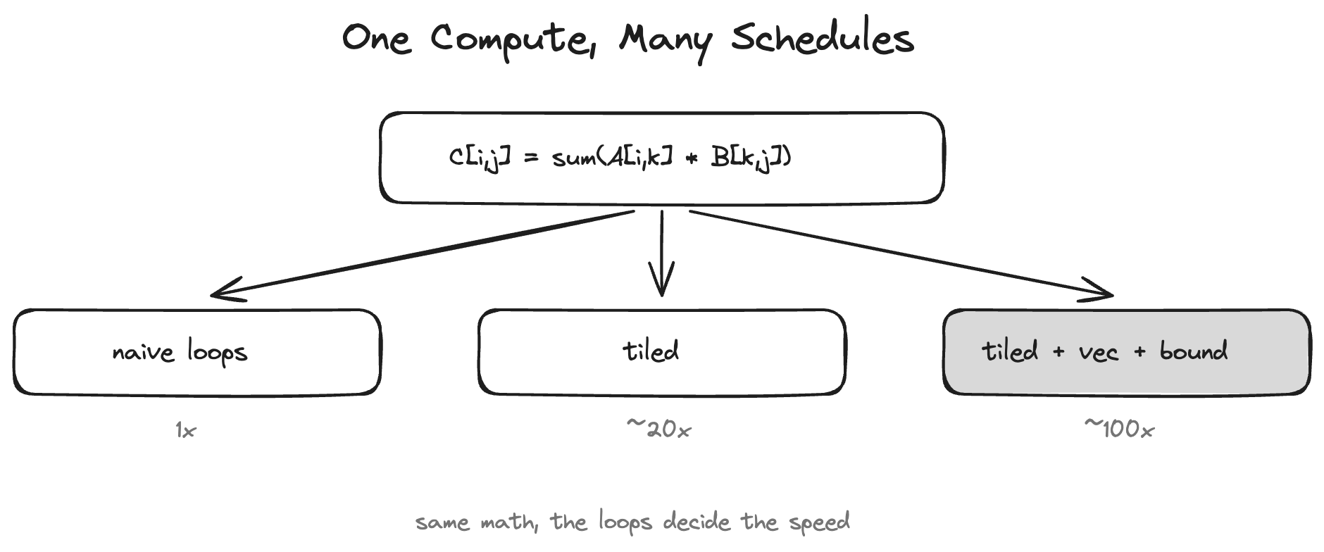
Day 6 - Loop Scheduling: Same Math, Different Speed

Compute/schedule separation: one compute definition, different schedules, kernels with wildly different speeds

Day 5 ended with a question: fusion decides which computations live in the same kernel, but what should the loops inside that kernel look like?

Here is why the question is worth money: the same math, written as different loop nests, can differ in speed by a factor of a hundred. A naive triple-loop matmul and the one inside cuBLAS perform exactly the same multiply-adds, yet sit two orders of magnitude apart. The gap does not come from "computing faster"; it comes from "moving less". This post is about how a compiler arranges that loop nest.

Reuse: Matmul's Natural Gift

Start with matmul's excellent constitution. Computing C = A × B (all N×N) takes 2N³ multiply-adds, but the inputs and outputs total only 3N² numbers. On average, every number gets used N times.

That is the high arithmetic intensity from Day 4. But note: it is a theoretical value. The naive loop looks like this:

for (i = 0; i < N; i++)
  for (j = 0; j < N; j++)
    for (k = 0; k < N; k++)
      C[i][j] += A[i][k] * B[k][j];

The problem is the revisit rhythm. The same column of B gets re-read in full every time i advances; by the time you need it again, it has long been evicted from cache by everything read in between. So "each number used N times" in theory becomes "fetched from HBM again on every use" in practice. Theoretical intensity is the constitution; how much you actually achieve is decided by the shape of the loops. Scheduling is the craft of closing that gap.

Tiling: Lock the Reuse Inside Fast Memory

The first and most important move: tiling (also called blocking).

The idea is simple: instead of computing whole rows at a time, compute one small block at a time. Cut C into T×T tiles; computing one tile only needs T rows of A and T columns of B. Pick T so that this working set fits in shared memory, and after one read from HBM, all T reuses of that data happen in fast memory.

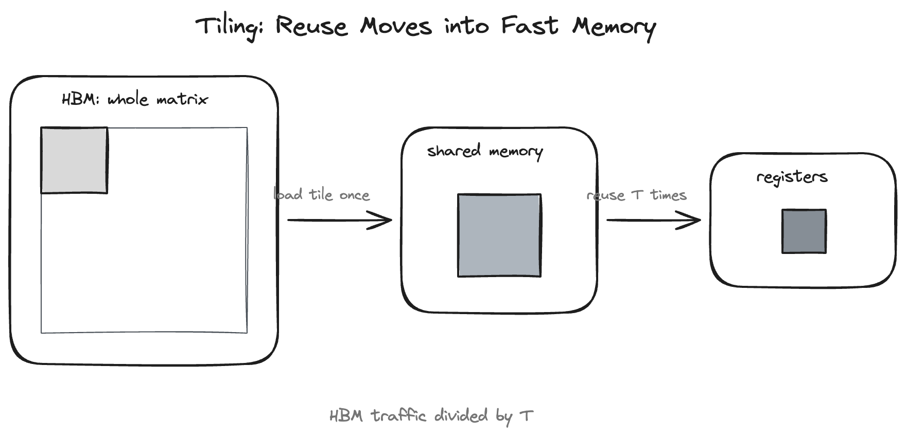
Tiling moves the reuse from HBM into shared memory and registers

The arithmetic is direct: without tiling, B gets read from HBM N times in total; with tile size T, only N/T times. HBM traffic divided by T. In practice this is done at two levels: one big tile from HBM into shared memory, then a smaller tile from shared memory into registers, matching the two big cliffs in the GPU memory hierarchy.

T cannot be chosen carelessly: too small and there is not enough reuse; too big and shared memory overflows, or occupancy drops (Day 5's register pressure applies here too). Park the question "how do you pick T"; it is the protagonist of the next post.

The Other Moves: Reorder, Vectorize, Unroll, Bind

Beyond tiling, a schedule has a few standard moves, each aimed at one concrete hardware reality:

Reorder. Choose which dimension sits in the innermost loop. The goal is to make innermost memory access contiguous: on a GPU, adjacent threads must touch adjacent addresses for accesses to coalesce (Day 3's layout story, replayed from the loop's point of view).

Vectorize. If the innermost loop accesses memory contiguously, one instruction can move 128 bits (say, four floats) instead of one element at a time. A quarter of the load instructions, much better bandwidth utilization.

Unroll. Replicate the innermost loop body a few times, shedding the loop's own compares and jumps, and handing the hardware more independent instructions to overlap. The cost is bigger code and more registers, another knob to balance.

Bind. On a CPU the loop really iterates; on a GPU, outer loops are flattened onto hardware: this level maps to thread blocks, that one to threads. Which level binds to what decides how parallelism and locality get distributed.

None of these four are abstractions: TVM's tir.Schedule exposes them as primitives under exactly these names, and you can apply them to a matmul's loops directly:

sch = tvm.tir.Schedule(matmul)
i, j, k = sch.get_loops(sch.get_block("C"))
io, ii = sch.split(i, factors=[None, 32])  # tiling, in loop form
jo, ji = sch.split(j, factors=[None, 4])
sch.reorder(io, jo, ii, k, ji)   # reorder: ji innermost, so access is contiguous
sch.bind(io, "blockIdx.x")       # bind: spread outer loops onto hardware
sch.bind(ii, "threadIdx.x")
sch.unroll(k)                    # unroll: drop the loop overhead
sch.vectorize(ji)                # vectorize: move 4 floats per instruction

Each move alone is easy. The hard part is that they entangle: tile size affects whether unrolling pays, reorder decides whether vectorization is possible, and binding constrains the tiles. A kernel's schedule is one set of coupled decisions, not four independent switches.

Separating Compute from Schedule

Now for the biggest idea in this post. Traditionally, CUDA engineers hard-wired all the moves above into the source: tile sizes, loop nesting, thread mapping, all tangled in one file. Want a different arrangement? Rewrite the kernel.

Halide, an image-processing language from 2012, proposed a different division of labor, later carried into the ML world by TVM: split "what to compute" and "how to compute it" into two descriptions.

Compute: pure math. C[i,j] = sum(A[i,k] * B[k,j], axis=k), one line, zero performance decisions.
Schedule: a list of transformations. "Split i and j by 32", "move k outward", "bind this level to blocks, that to threads", "vectorize the innermost loop".

The key guarantee: a schedule changes only execution order and data placement, never the result. Every schedule primitive (split, reorder, bind, vectorize...) is a semantics-preserving transformation.

This separation buys three things. First, courage: since no arrangement can be wrong, you can try wild ones; the worst case is slow, never incorrect. Second, portability: one compute definition, one schedule for GPU, another for CPU, another for next year's accelerator; the math is written once. Third, and most far-reaching: the schedule becomes data. No longer a style buried in source code, but an object that can be enumerated, compared, and searched.

Conclusion

To close: a kernel's speed is decided not by its math but by the shape of its loops, because that shape determines how much of the theoretical reuse actually happens in fast memory. Tiling locks reuse into shared memory and registers, reorder and vectorize make every trip smoother, unroll and bind spread the parallelism across the hardware. And compute/schedule separation turns all of this from craft hard-wired in code into an object you can manipulate on its own.

Next Up

If schedules are objects, they can be searched. But how big is the space? Tile sizes, loop orders, unroll factors, binding choices, all multiplied together is astronomical, and the answer changes with every op, every shape, every GPU. Day 7 covers auto-tuning: how machines find good schedules in that space, and why the cost model is the heart of the whole business.