Day 6 ended by turning the schedule into "an object that can be searched". This post does the searching.
First, feel the size of the space. A matmul schedule must decide: tile sizes at two or three levels (a dozen choices each), loop order, unroll factor, vector width, which levels bind to blocks and threads, whether to stage through shared memory. These choices multiply, easily reaching millions to billions of combinations. And the answer does not transfer: change the shape (512×512 to 4096×4096) or the GPU (A100 to H100), and the optimum moves. It is a problem that must be re-solved in every cell.
The Limits of Hand-tuning
The traditional answer is people. cuBLAS and cuDNN are the extreme of that road: vendor engineers hand-tune near-peak kernels for every hardware generation and every common shape, shipped as a library.
Two ceilings. First, only the popular cells get covered: common shapes get expert attention, long-tail shapes (odd dimensions, small batches) make do with an ill-fitting version. Second, and fatal for compilers: fused kernels have no library. Day 5's fused kernels are stitched together on the fly, following the specific model in front of the compiler; their shapes are one-of-a-kind, and nobody could have pre-tuned them. If the compiler generates its own kernels, it must solve its own schedules.
Turning It into Search
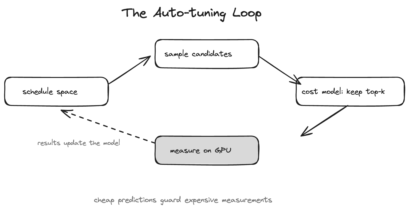
Auto-tuning is a loop with four roles:
The search space. Define which schedules are legal candidates. Early AutoTVM used templates: engineers wrote the schedule skeleton, leaving knobs like tile sizes for the machine to turn. Ansor and MetaSchedule went further, generating the skeletons themselves from rules, no templates required. Triton's autotune and torch.compile's max-autotune mode pick among a set of pre-written configs.
The sampler. Pull a batch of candidates from the space. Pure random is wasteful; the usual choice is evolutionary search: seed with the best schedules known so far, mutate and cross-breed the next batch.
The cost model. The heart, next section.
Real measurement. Actually compile the kernel, run it on the GPU, time it. The only source of truth, and the most expensive: one measurement costs milliseconds to seconds, and occupies the hardware.
One turn of the loop: sample a batch → cost model scores them fast, keeps the top few → only those run on real hardware → measurements feed back to update the model → next round's sampling and scoring get sharper.
The Cost Model: Trading Prediction for Measurement
Why is the cost model non-negotiable? Do the arithmetic: the space starts at millions; even at 10ms per measurement, measuring everything takes hours to days, and that is one kernel. Not viable.
The cost model's role is cheap approximation: given a schedule's features (tile sizes, access patterns, parallelism...), predict its speed in microseconds. Does it need to be accurate? Not very; getting the ranking right is enough: its job is not to report correct milliseconds but to pick, out of a thousand candidates, the ten worth measuring.
Better yet, it learns as the search runs. Every real measurement is a fresh training example, and the model grows to know the temperament of this particular GPU. That is the trade: cheap predictions standing guard in front of expensive measurements. The efficiency of the whole enterprise rests on this layer.
TVM MetaSchedule
The four roles are an abstract frame; in TVM's MetaSchedule (recently refactored into s_tir/meta_schedule/), one round of search runs like this.
The initial population is 512 traces from two sources: twenty percent are the best measured records pulled from the database as seeds (PickBestFromDatabase), the rest are randomly generated (SampleInitPopulation). Then four rounds of evolution: each round, the cost model scores the whole population; scores become sampling probabilities for picking parents; with 85% probability a mutator is applied (swap a tile size, change unroll depth, adjust parallelism); the mutated trace must still pass postproc validation, with up to ten retries on failure. Schedules already measured are filtered out by IRModule hash, so they never re-enter the candidate heap.
After four rounds, the picks are not purely greedy: PickWithEpsGreedy takes 95% from the top predicted scores and mixes in 5% random candidates. That 5% is insurance: if the cost model keeps misjudging one direction, pure greed would forever steer around that unexplored region.
The chosen candidates go to the builder for compilation and the runner for measurement (over RPC to remote devices if needed), and a measure callback writes results into two JSON files: database_workload.json for the workloads, database_tuning_record.json for each trace and its time. That is the physical form of the "lookup table" from the previous section. The same callback retrains the cost model, so the next round's scoring is sharper.
The cost model itself is XGBoost. Its features are not raw code but a vector extracted per buffer store: counts of each arithmetic op class, reuse patterns and strides of buffer accesses, the arithmetic intensity curve, allocation sizes, outer loop structure. The training target is worth noting too: it learns not "how many milliseconds this schedule takes" but a normalized relative throughput. Which echoes the previous section: getting the ranking right is enough.
PyTorch max-autotune
Switch to PyTorch Inductor (torch/_inductor/) and something interesting appears: GEMM tuning under mode="max-autotune" has no cost model at all.
Because its space is several orders of magnitude smaller. Inductor does not generate schedules; it enumerates backends × configs: ATen (calling straight into cuBLAS), Triton templates (the plain one, a persistent TMA one, a Blackwell warp-specialization one), CUTLASS, ROCm's CK, a C++ GEMM template for CPU, plus a few subgraph tricks such as decompose_k, which splits a long-K matmul into batches and sums. Each template's configs are pre-filtered by heuristics on hardware and shape; the default tier keeps a few dozen candidates. A few dozen candidates: just measure them all. Measurement itself is the cost model.
The engineering effort goes into making measure-everything fast and safe instead: candidate kernels precompile in parallel on a thread pool, and benchmarking can run in a separate subprocess pool (autotune_process.py), so one config crashing CUDA cannot take down the main compile process.
There is pruning between candidates too. At large K, decompose_k nearly always wins, so the Triton template simply stays off the candidate list; the comment in kernel/mm.py is blunt about Triton being highly unlikely to ever win there. That is human prior knowledge cutting the space, versus a cost model cutting it with learned knowledge: two versions of the same move.
After a Triton config wins, one more finishing pass: coordinate descent tuning. Knobs like BLOCK_M, BLOCK_N, num_warps move one at a time, one neighborhood step per move, keeping whatever improves. Global search picks the template; local hill-climbing polishes the config; each layer owns its stretch.
On the lookup-table layer Inductor goes further still: beyond the local cache there is a remote cache so a whole cluster shares tuning results, and there is now even a lookup table that maps hardware + shape + op straight to a template config, bypassing search entirely.
Side by side, these are the frame's two extremes: MetaSchedule's space is generative, starting at millions, so the cost model is the heart; Inductor's space is enumerative, capped at dozens, so it skips the cost model altogether. How you define the space decides the entire technical road. That is the real weight of Day 6's "schedule space" abstraction.
The Ledger of Tuning
Auto-tuning is not free, and its yield curve looks like this:
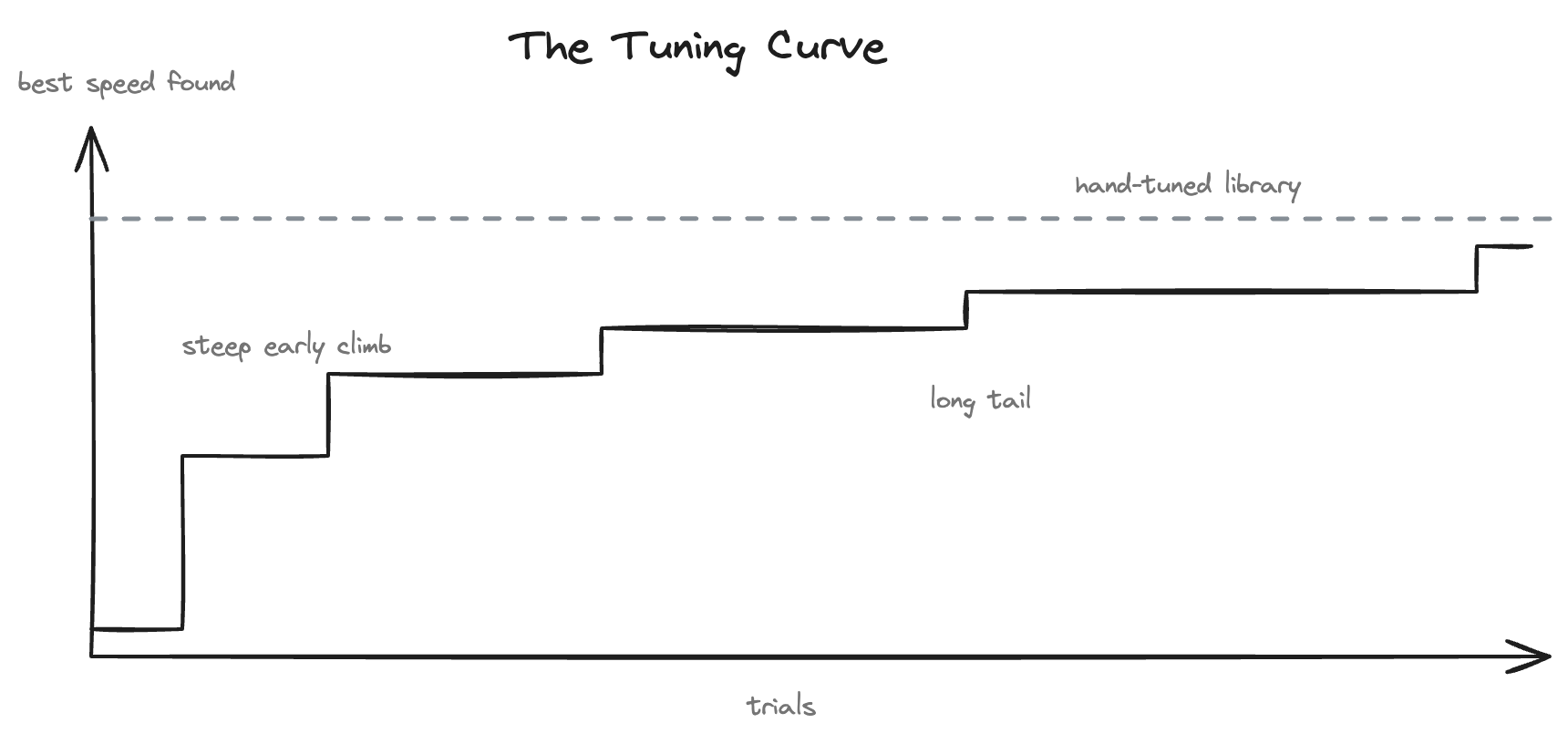
The first few dozen candidates usually match a naive implementation; then comes the long tail: minutes to hours of search, slowly approaching and sometimes beating the hand-tuned library. Whether it is worth it depends on how many times the kernel will run: in an inference service where one kernel is called hundreds of millions of times a day, an hour of tuning is obviously a bargain; for research code that runs once, the default schedule is fine.
So mature systems store their tuning results: TVM's tuning logs, torch.compile's cache, all essentially a lookup table from (op, shape, hardware) to best schedule. Tune once; every later encounter with the same combination is a table lookup, and the cost amortizes to zero.
Hence the different gears: torch.compile defaults to heuristics (fast, no search), and only mode="max-autotune" unleashes the full search. It is a slider trading compile time for run time; where you set it depends on your scenario.
Conclusion
To close: the schedule space is so large that human hands only cover the popular cells, and compiler-fused kernels have no library at all, so search is inevitable. The framework is a loop of four roles: space, sampler, cost model, measurement. The heart is the cost model, microsecond predictions standing guard before second-scale measurements, reducing a space of millions to a few hundred real runs. The key to the ledger is amortization: results are banked by (op, shape, hardware), and the more you run, the better the deal.
Next Up
Notice the assumption hiding throughout this post: fixed shapes. Results are banked per shape, tiles are chosen per shape; all the goodness rests on knowing tensor sizes at compile time. But in real LLM serving, every request has a different length. Day 8 covers dynamic shapes: which parts of static compilation collapse when shapes move, and the three ways to catch them.